
For those of you who have asked — in person, in DMs, after a talk — what the UYIR paper is actually about, this is my honest attempt to explain it without the equations, without the appendices, without the part where I quietly hide how surprising the answer turned out to be.
Let me start with the question I actually asked. What if a language model had life?
Not life in the the model is conscious sense — that is a different conversation and one I am not the right person to have. I mean it in the small, technical, slightly biological sense: what if the parts of a model — the tiny low-rank adapters that we layer on top of a frozen backbone to specialise it — were treated as a population? Adapters that compete on a fitness signal. Adapters that get killed if they aren't pulling their weight. Adapters that reproduce by cloning the fittest one and adding a little mutation noise to keep the gene pool fresh. Adapters that, on their way out, blend a fraction of their weights into their nearest neighbor — a kind of last-breath inheritance, so the population doesn't lose what they spent their short lives learning.
I have wanted to build this for years. The hypothesis, in one sentence: lifecycle dynamics — selection, reproduction, inheritance, mutation — should produce better-organized adapter populations than static allocation does, because that is the entire premise behind why biology works.
The name I gave the system is UYIR — உயிர், the Tamil word for life. It stands, loosely, for Unit-level Yield-driven Inheritance and Reallocation, which is just the four ingredients spelled out: operate at the unit of a single adapter, drive decisions by counterfactual yield, blend a dying adapter into its nearest neighbor, and reallocate the vacated slot to a mutated clone of the fittest. The acronym worked out almost too cleanly, which should probably have been a warning.
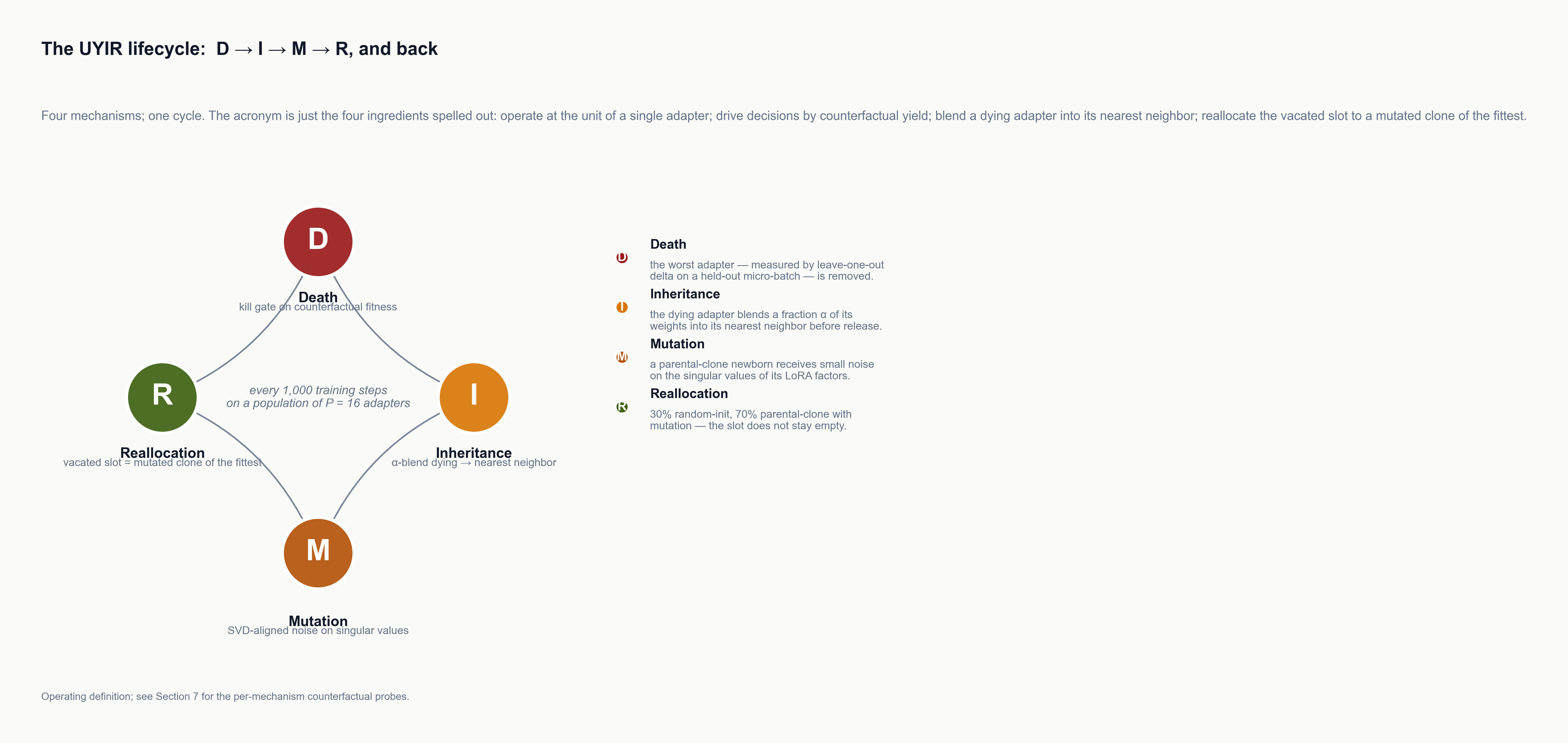
The paper I just submitted to TMLR — Decomposing Evolutionary Mixture-of-LoRA Architectures: The Routing Lever, the Lifecycle Penalty, and a Substrate-Conditional Boundary (arXiv:2605.11153) — is, in part, a love letter to that idea. It is also, mostly, a careful and slightly painful exercise in what happened when I asked the data whether the idea was true.
What I wanted the answer to be
I will admit this upfront because it shapes everything that follows: I wanted the answer to be yes. I wanted the lifecycle to pay rent. I wanted the adapters to evolve, to specialise, to organize themselves into domains, and for the resulting model to beat a static baseline by a margin that vindicated the months I had spent on it. I wanted the picture to look like the cover image I had in my head: a phylogenetic tree of adapter populations, branching and dying and re-flowering across training, the whole thing visibly alive.
I did not get the answer I wanted. I got a more interesting one.
The actual question, the one I had to pin down
If you build something like UYIR — a population of LoRA adapters under a router, with a lifecycle loop on top — and you train it next to a static mixture-of-LoRA baseline, and it improves the held-out perplexity by some amount, how do you know the improvement came from the lifecycle? The honest answer is: you don't, not without taking the system apart and testing each piece against the same statistical bar as the whole.
So that is what I did. I decomposed the system into three factors:
- F1, the router. The legacy softmax router with token-embedding input, vs. a rewritten router: a parallel-sigmoid gate with a learnable per-adapter floor and a bounded temperature anneal, fed not the token-embedding mean but the post-stack hidden state of each token. (This is a much smaller change than it sounds; it is roughly fifty lines of code.)
- F2, the evaluation scope used by the selection signal. Either an aggregate cross-domain held-out loss, or a per-domain leave-one-out signal that asks "what does the population look like with this adapter removed?"
- F3, the lifecycle bundle. Death, $\alpha$-blend inheritance, SVD mutation, and slot reallocation, on or off as a single unit.
Three on/off factors means a full factorial is $2^{3}$ = 8 cells, but I budgeted for the five cells that let me reconstruct the attribution chain at $n{=}3$ seeds per cell, $25{,}000$ adaptation steps each. That is 15 production runs. I pre-registered the decision rules, pinned the sign convention and the aggregator (geometric mean of per-domain perplexities), and committed everything to a frozen hash before launching the first cell.
I want to flag that last detail because it ends up mattering. The decision rules were locked before any cell ran. When the data came back, I did not get to retune the thresholds. I got to read the verdict.
What the decomposition actually showed
The headline-level result was the first thing that confused me.
The full-system-vs-baseline contrast at $n{=}3$ seeds — the did the whole thing help number — came in at $+0.015$ nats balanced log-PPL, $t{=}1.94$, $p{=}0.19$. Not significant. The improvement I had hoped to celebrate was, statistically, a wash.
This is the moment in a normal research paper where you write "more work is needed" and quietly move on. But the decomposition was already running, and the decomposition told a much sharper story. Inside that $+0.015$-nat headline, two competing effects were nearly cancelling:
F1 — the router rewrite — contributed $+0.0426$ nats by itself, $t{=}12.86$, $p{=}0.006$. A large, robust, structurally significant effect. The kind of effect you would name a paper after.
F3 — the lifecycle bundle — contributed $-0.028$ nats on top of F1, $t{=}-4.46$, $p{=}0.047$. A net drag. The evolutionary machinery I had built was, on this substrate, actively hurting the model that the router rewrite had already improved.
F2 — the per-domain evaluation scope — was null at seed resolution.
I read those numbers a few times. I re-ran the attribution chain through a second, non-overlapping consistency path through the factorial — different cells, different intermediate steps, same input data — and the two chains converged on the lifecycle penalty to within 0.0004 nats ($-0.0283$ vs $-0.0287$) and on the router contribution to within 0.001 nats ($+0.0426$ vs $+0.0436$). The decomposition was internally consistent. The conclusion was uncomfortable.
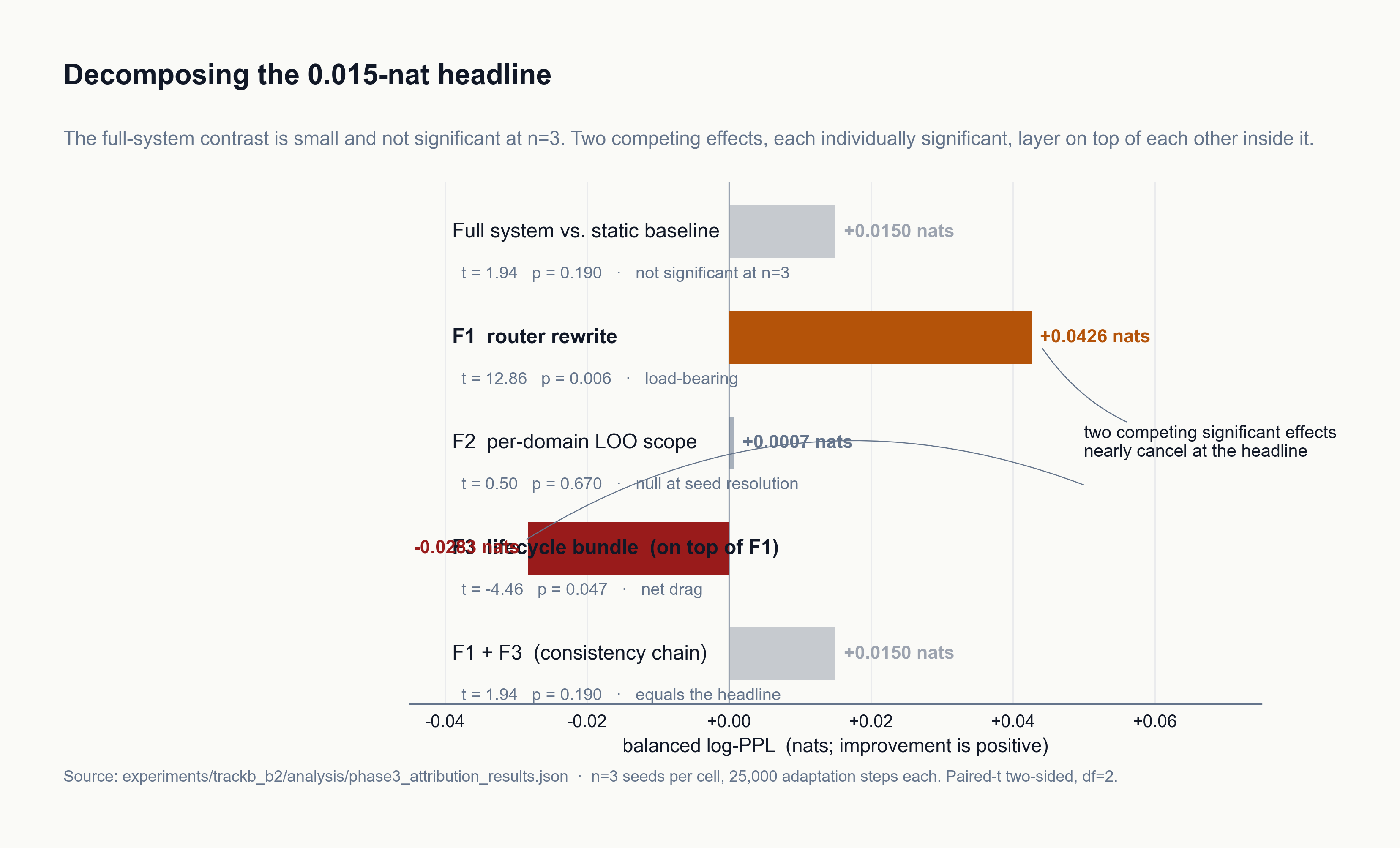
The thing I had built UYIR around — the lifecycle — was anti-aligned with the gradient solution that the router rewrite unlocked. The thing I had thought of as plumbing — a router fix I almost did not bother to factor into the design space — was carrying the entire signal.
The router rewrite, or: why the legacy gate was secretly broken
Once it was clear that F1 was where the action was, I had to understand why. I am not interested in shipping a paper that says "this thing worked" without an account of what it was doing. So I went and looked at what the legacy softmax router was actually computing.
What I found was almost embarrassing. On this substrate, the softmax-over-adapters router was collapsing onto a single 4-of-16 cross-domain adapter coalition — adapters ${0, 6, 8, 12}$, the same four, at every layer of every sample. Every domain — biology, code, general text, scientific writing — was being routed to the same four adapters. The other twelve received zero routing mass; effective capacity utilisation was $25%$. The per-domain top-$k$ gate distributions had Jensen–Shannon divergence exactly zero across all ten domain pairs. That is not low — it is a hard-zero indicator that the four gate distributions are identical. The router was not specialising. It was monopolising.
The part that made it unambiguous — that this was the router's failure and not the substrate's — was a control. The substrate plainly carried domain signal: the per-domain gradient-norm Jensen–Shannon divergence reached $3.88$ for the code↔science pair, roughly $31\times$ the narrow-baseline value of $0.126$. The information needed to route was right there in the hidden states. The router simply was not routing on it. And the coalition was structurally locked: forcibly killing one of its four members at step 4000 did not dislodge the router from the same identity set — it just re-formed around the survivors. A monopoly that heals itself when you shoot one of its members is not a thing you fix by waiting.
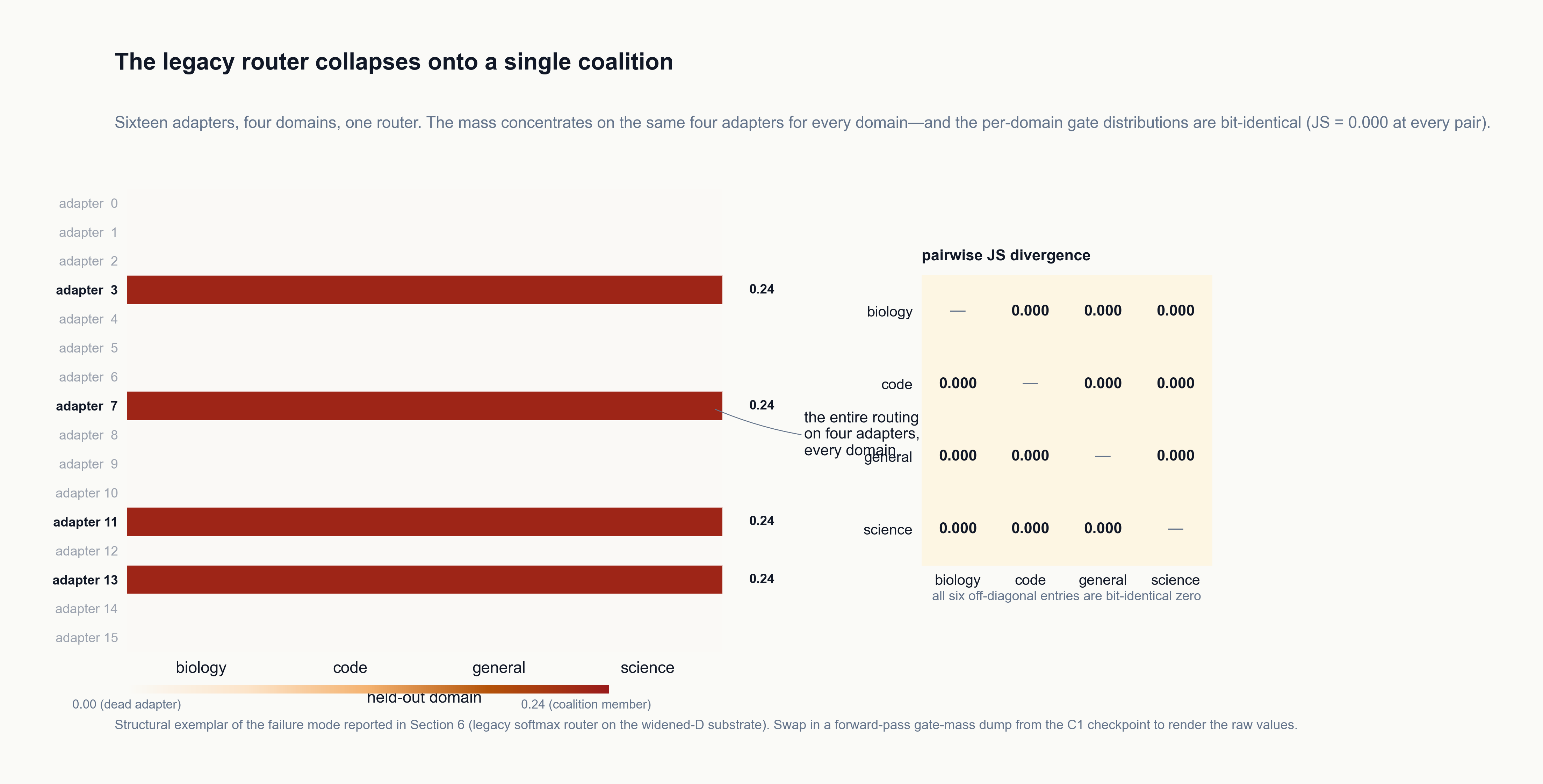
I had been training a population of sixteen adapters and the router was using four of them, for everything, all of the time, with no per-domain differentiation at all. The other twelve adapters were dead weight from the router's perspective. The fact that the system still managed to learn something was a kind of slow miracle of LoRA's natural averaging.
The rewrite fixed this in three structural moves, each small on its own:
- A parallel-sigmoid gate instead of a softmax. Softmax forces the gate values to sum to one — they are competing for a fixed budget, and that competition is what creates the monopoly. A parallel sigmoid lets every adapter's gate be in $[0,1]$ independently. Lifting one gate no longer mechanically depresses the others.
- A learnable per-adapter floor. A small per-adapter minimum that the gate cannot collapse below. This stops the "dead adapter" failure mode in which the router never assigns mass to an adapter, so the adapter never receives gradient, so it can never become useful — a classic mode-collapse.
- A different input. Instead of feeding the router the mean of the token embeddings, which loses almost all per-domain signal by design, feed it the post-stack hidden state of each token. This is, by a factor of about $20\times$, a more domain-differentiating signal than the embedding mean.
The three changes are not independent. The sigmoid alone, on the embedding-mean input, is not enough — there is nothing for it to differentiate on. The hidden-state input alone, under softmax, still gets squeezed into a monopoly because softmax is the structural problem. The combination dissolves the monopoly. Every held-out domain — biology, code, general, science — improves under the rewrite, not just the balanced aggregate.
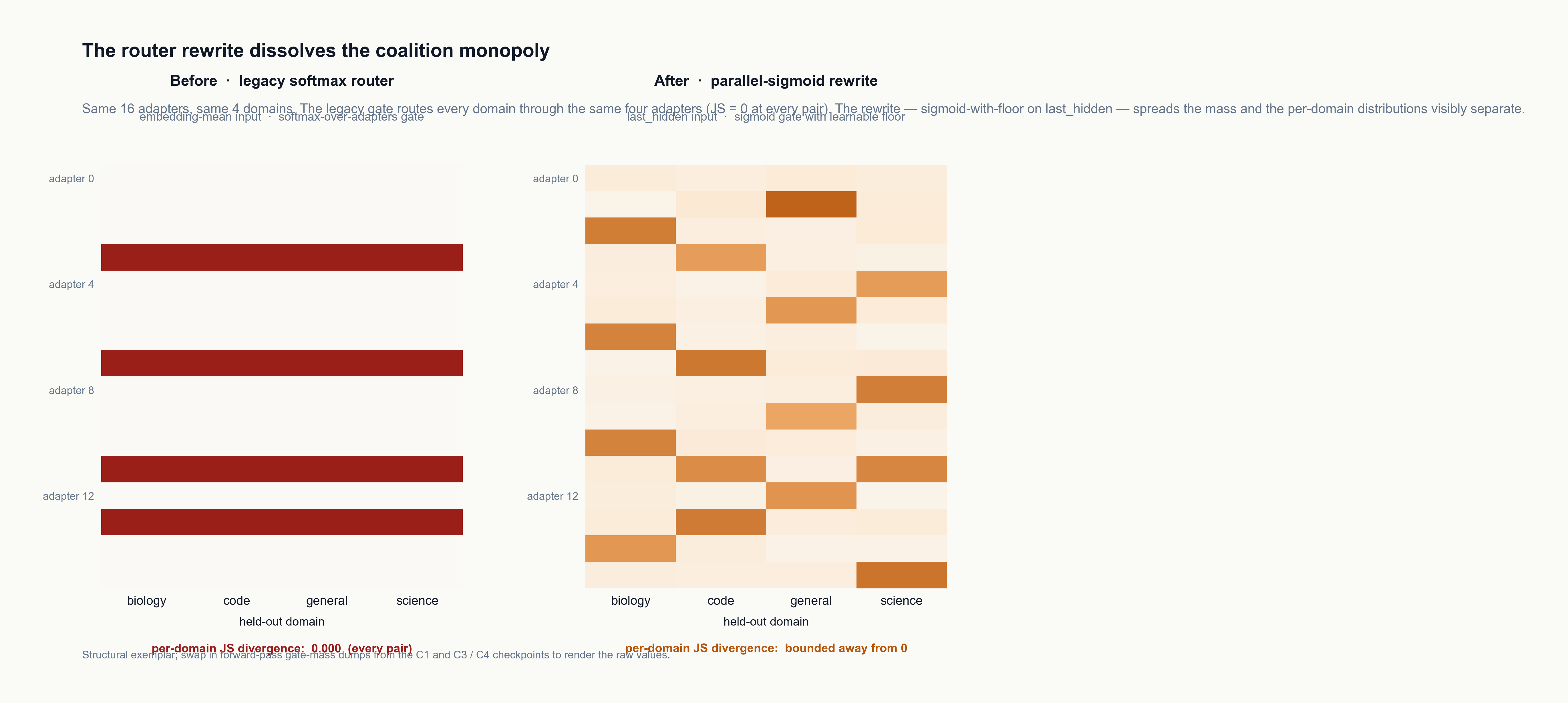
The paper has the full mechanism walkthrough. The thing I want to flag here, for anyone building a mixture-of-LoRA system from scratch, is that the legacy router is the kind of thing you do not look at until it is too late, and looking at the Jensen–Shannon divergence between per-domain gate distributions is a five-line probe that would have saved me six months. The exact-zero result is not a number you usually see in machine learning. When you see it, something is wrong.
Where the lifecycle penalty actually lives
Once F1 was characterised, the harder question was: F3 is a bundle of four sub-mechanisms — death, inheritance, mutation, reproduction. Which of them carries the $-0.028$-nat penalty?
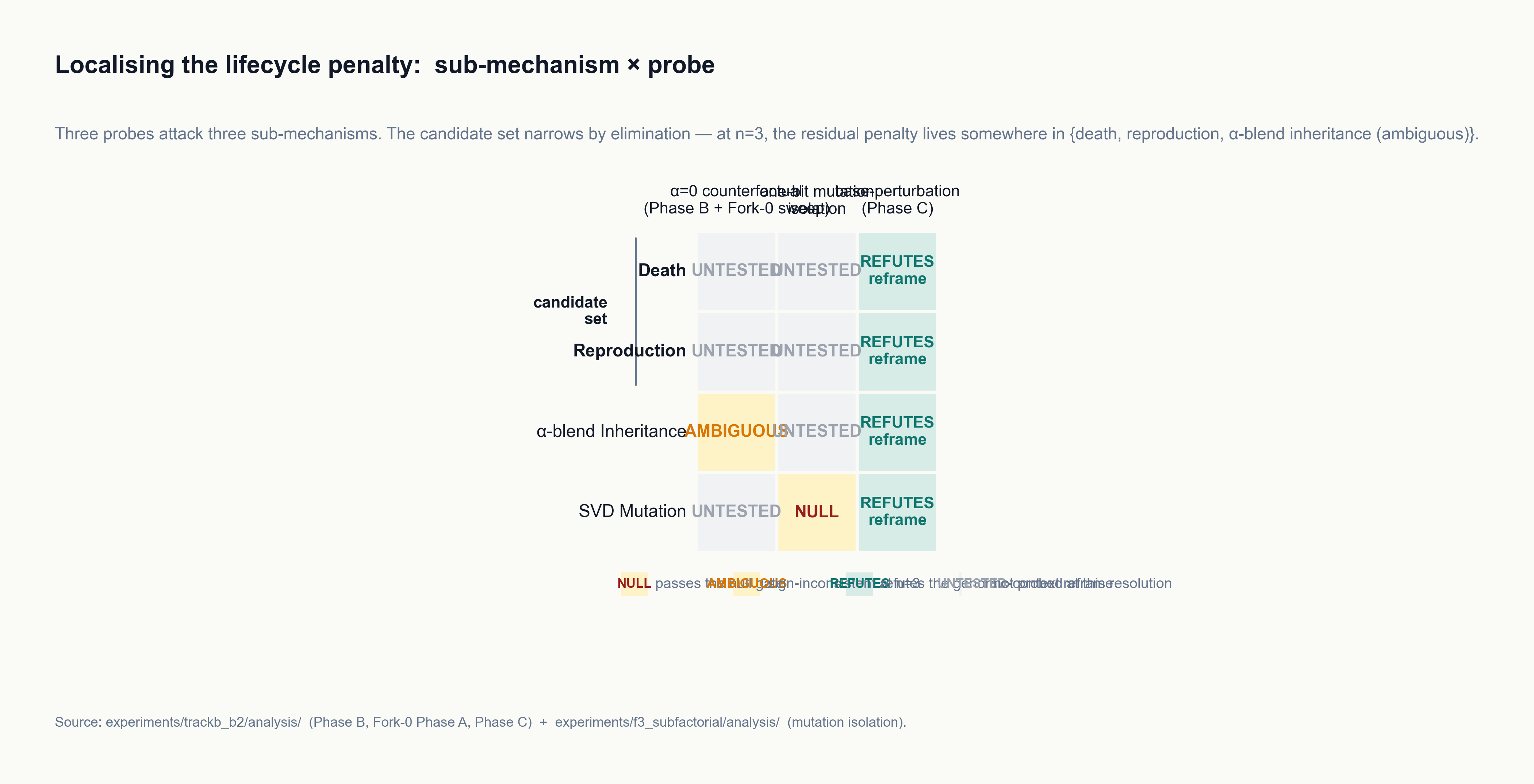
I ran three independent probes, each attacking a different sub-component, before submitting the paper:
The inheritance counterfactual — re-running the winning cell with $\alpha{=}0$ (inheritance off) — was the cleanest test of the "I" in UYIR. At $n{=}3$ seeds the per-seed shifts were $+3.18%$, $-1.65%$, $+0.20%$. The signs are inconsistent. The cross-seed mean is $+0.56%$, well inside the ambiguous band of the pre-registered decision rule. Ambiguous at $n{=}3$. I had wanted a clean equivalence verdict here — "inheritance is decorative" would have been a useful negative result — but the data refused to commit either way. The inheritance counterfactual remains suspect, neither cleared nor convicted.
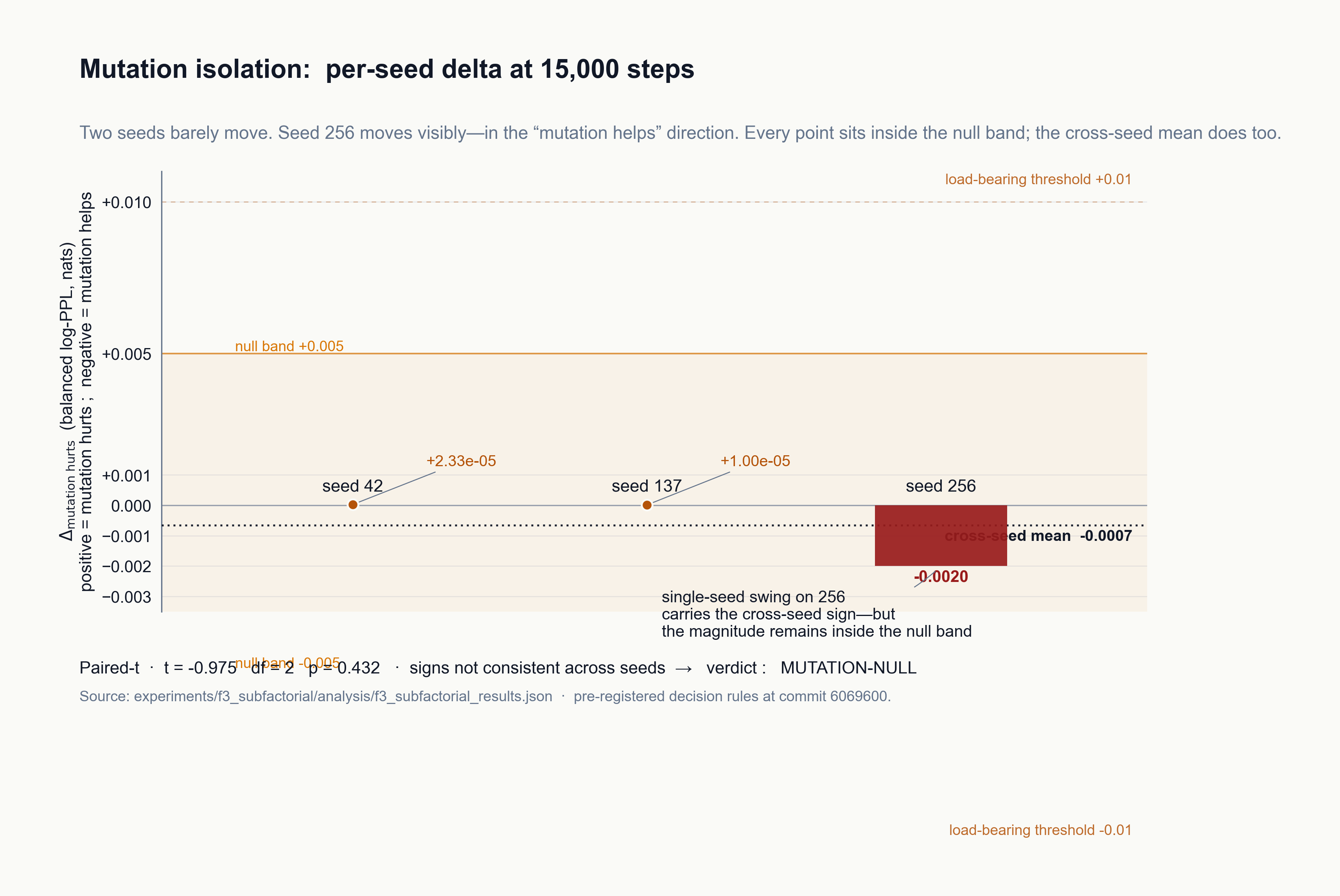
The mutation isolation — a one-bit sub-factorial that holds $\alpha{=}0$ and compares death-plus-reproduction with mutation off (S-DR) against death-plus-reproduction with mutation on (S-DRM), six cell-seed runs in total — was the test of the "M" sub-component. The verdict was MUTATION-NULL. Across three seeds, the paired shift in balanced log-PPL was $-6.6 \times 10^{-4}$ nats, paired-$t$ $p{=}0.43$, signs not consistent. Mutation, on this configuration, is not load-bearing. The SVD-aligned perturbation operator that I had spent weeks polishing was, statistically, contributing nothing.
The base-perturbation probe — hot-swapping the trained adapter population into earlier checkpoints of the base model — was the test of a more exotic alternative hypothesis: that adapter specialisation might be carried by the base model's internal representation rather than the LoRA delta itself. (Call it the genomic-context reading: the adapters are the proteins, the base is the genome, and what survives is information about the genome.) If that reading were correct, adapter fitness differentiation should expand when the base is rolled back. The variance ratio at off-canonical bases came in at 0.15 — a $7\times$ inversion in the wrong direction. Bootstrap 95% CI excludes 1.0 by orders of magnitude. The genomic-context reframe is refuted. The adapter specialisation is real but co-adapted with the canonical base; it is not transferable across base eras.
So: mutation null, inheritance ambiguous, genomic-context refuted. By elimination at $n{=}3$, the damaging contribution lives in some subset of death (the kill gate's selection on counterfactual fitness), reproduction (the placement of new adapters into vacated slots — $30%$ random-init, $70%$ parental-clone), and — pending the still-ambiguous inheritance counterfactual — $\alpha$-blend inheritance. The probes constrain. They do not pin.
I would love to tell you that I have an elegant story about which of death or reproduction is the culprit. I do not, yet. That is the broader $2^{3}$ sub-factorial that lives at the top of my next-experiments queue.
The synthetic boundary, or: why this was always going to be hard
Running parallel to the production-substrate factorial, I built a small, controllable, synthetic sandbox — vocab 128, four disjoint slabs, deterministic bigram, hidden 512, sixteen LoRA adapters with top-$k{=}4$ — where the ground truth is known and I can ask whether evolutionary search on the routing channel is load-bearing at all, anywhere, under any condition I can construct.
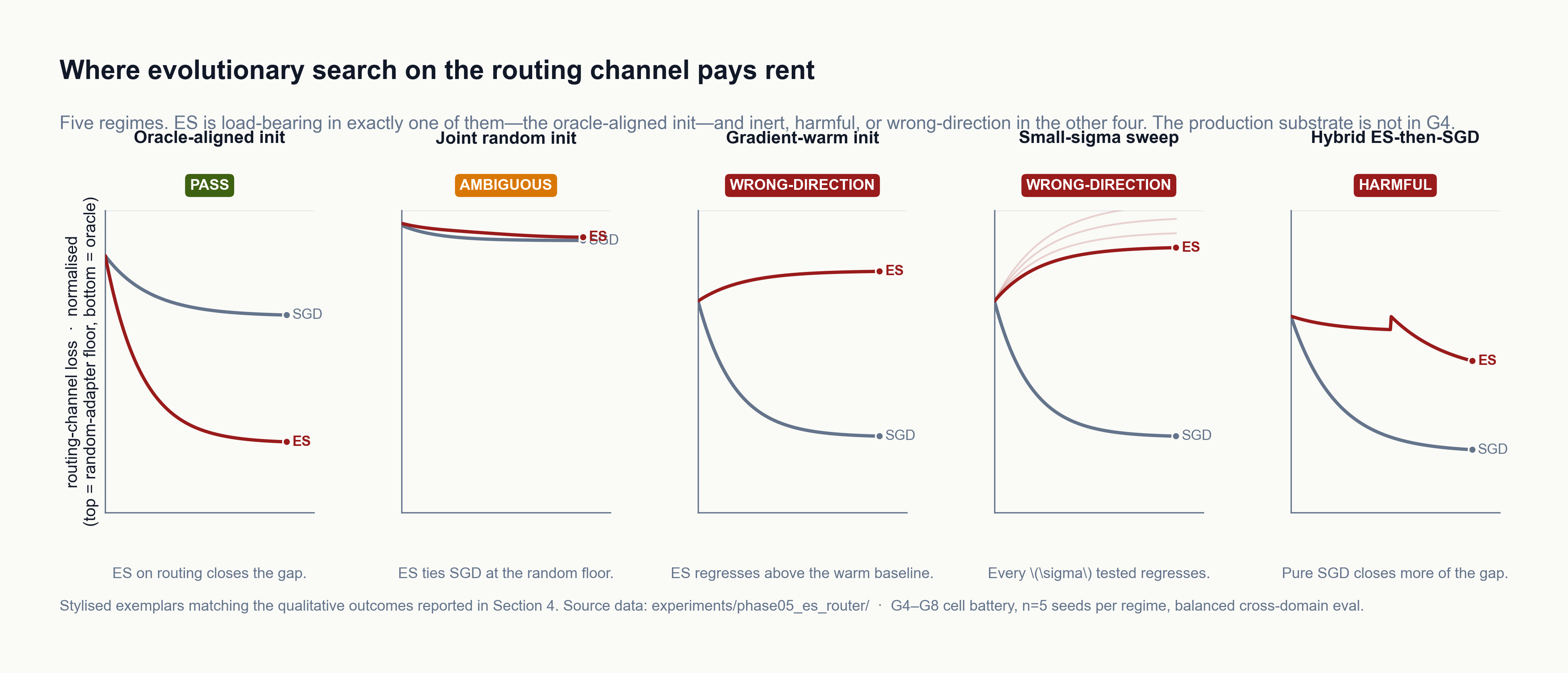
The sandbox produced one of the cleaner regime characterisations I have ever measured. Across five experiments — G4 (oracle-aligned adapter initialisation), G5 (joint random initialisation), G6 (gradient-warm initialisation), G7 (small-sigma evolutionary search), G8 (hybrid ES-then-SGD schedules) — evolutionary search on the routing channel is load-bearing only in G4, the regime where adapters are pre-aligned to the per-slab oracle solution. In every other regime — joint random init, gradient-warm init, hybrid schedules at every $\sigma$ and interleave we tested — evolutionary search underperforms, ties, or actively degrades the gradient solution.
This is not a small caveat. It is, in retrospect, the prior I should have looked at before I started building UYIR. The production substrate is not in the oracle-aligned regime — there is no oracle pretrain, adapters are randomly initialised at the start of adaptation, the router and the adapters co-evolve under the same next-token gradient. The synthetic sandbox predicts, before any production-substrate measurement is consulted, that the production lifecycle outcome should resemble G5–G8 (small effect, inert, or harmful) more than G4 (load-bearing).
The production F3 outcome — a $-0.028$-nat net drag — is exactly that prediction. The sandbox and the production substrate are telling the same story, in two different vocabularies. The lifecycle did not fail because I implemented it wrong. It failed because the substrate was not in the regime where evolutionary search on the routing channel can pay rent. Knowing that — having a sufficient condition that I can point to and say here is where this might work — is, perversely, the most useful thing the paper contains.
A word on the substrate, and its two scars
I have been saying "on this substrate" a lot, and it is worth being concrete about what the substrate is, because two scars in it shaped everything that followed. It is a from-scratch GPT of about $150$M parameters, $D{=}1536$, vocabulary $V{=}32{,}000$, frozen for adaptation at pre-training step $70{,}000$.
The width was deliberate. When $D \ll V$, backpropagating $V$-dimensional gradients through a rank-$D$ output projection destroys most of the gradient norm — at $D{=}768$ over a 32K vocabulary, on the order of $98%$ of it — and every adapter downstream is then trying to learn from a badly degraded signal. Widening to $1536$ was the fix. It is also the reason the $F1$ routing-input change (embedding-mean → last-hidden) carries roughly $20\times$ more cross-domain signal on this substrate than it would on a narrow one — which means $F1$'s load-bearingness is itself partly a property of the substrate I chose.
The step-$70{,}000$ freeze was not deliberate. The base was meant to train to roughly step $143{,}000$; a UPS power event killed pre-training partway, and I elected to ship the abbreviated base rather than restart a multi-day run. I mention it because it is the kind of thing that quietly never makes it into a paper, and it is exactly the kind of thing that makes a result substrate-conditional rather than universal. Both scars are substrate facts, not laws of nature. That word — substrate-conditional — is in the paper's title for a reason.
What I learned, what was new, what was sobering
A few things I want to write down explicitly before the post-submission haze rewrites them.
The new thing, the thing I had not seen written down anywhere I could find, is the JS-divergence-exactly-zero diagnostic for the coalition monopoly. It is not a fancy probe; it is one matrix multiplication. But it surfaces, in five lines of code, a structural failure mode of softmax-over-adapters routing that I had been chasing through perplexity curves for weeks before I thought to look at the gate distributions directly. The exact-zero is the tell. I expect this to be useful to anyone building a sparse-MoE-over-LoRA system, and I am much more interested in publicising it than the lifecycle finding.
The surprising thing was the magnitude of F1 vs F3. I had built F3 over months. I had built F1 as housekeeping — a small refactor to a routing module I considered solved. The numbers reversed my prior almost completely. The five-day refactor was the load-bearing piece. The six-month build was the drag. The lesson is the standard one — if you cannot make yourself look at the housekeeping, the housekeeping is where your bugs live — but it lands harder when it is your own work.
The sobering thing was the lifecycle penalty itself. I had a hypothesis. I tested it with discipline I am proud of (pre-registered rules, frozen hashes, source-of-truth conventions, paired-$t$ at $n{=}3$). The hypothesis did not hold. There is a particular kind of intellectual weight that comes with putting that result in a paper rather than burying it — and I want to be honest that I considered burying it. I have written drafts of this story where the headline is just F1 and the lifecycle penalty is a footnote. Those drafts felt wrong. The decomposition is the contribution; the decomposition only works if I report what it says.
The methodological thing — which I half-knew already but which this paper crystallised — is that the most important infrastructure work in a project like this is the audit chain. Every numerical claim in the paper traces to a single source-of-truth JSON file. The geometric-mean aggregator is pinned at the top of the evaluation section and is the only blessed path. The paired-$t$ tests on the headline are re-derived from per-seed JSONs, not from rolled-up summary files that can drift. None of that is glamorous. All of it is the difference between a paper that survives reviewer scrutiny and a paper that does not.
Two details make that concrete, and one of them is mildly humiliating. The decision rules were committed to frozen git hashes — 92c8637 and 6069600 — before any cell ran, so when the data came back I read a verdict rather than tuned a threshold. And the replay script refuses to emit a result at all if the geometric-mean and arithmetic-mean aggregators ever coincide — a mechanical tripwire against the exact aggregator confusion that, in an early version of this very result, made the lifecycle look like a twelve-sigma win. It was not twelve sigma. Under the correct geometric-mean convention the coherent paired-$t$ was $t{=}2.02$, $p{\approx}0.18$ — borderline, not triumphant. Catching that before submission, because the tripwire fired, rather than after, because a reviewer did, is the entire reason the audit chain exists.
What I want to do next, if I get the chance
The paper closes one loop and opens several. The ones I am most excited about, in roughly the order I will run them:

The broader $2^{3}$ × $\alpha$-toggle sub-factorial. The mutation-isolation result rules out mutation; the inheritance counterfactual is ambiguous; by elimination the lifecycle penalty lives in death and reproduction. A ten-cell partial $2^{3}$ over {death on/off, mutation on/off, reproduction warm/cold} crossed with ${\alpha{=}0.0, \alpha{=}0.2}$, at $n{=}3$ seeds per cell, $25{,}000$ adaptation steps, with persistent checkpoints throughout, would pin where the damage actually lives. Cost: about ~33 GPU-hours total on a single L40S. Three months from now I would like the paper to have a follow-up that says, finally, which of the four sub-mechanisms is the load-bearing one.
The F1 sub-factorial. F1 as run pairs two changes — the gate function (softmax → sigmoid-floor) and the routing input (embedding-mean → last-hidden). A four-cell sub-factorial, ${$softmax, sigmoid-floor$} \times {$embed-mean, last-hidden$}$, at $n{=}3$, would tell me which of the two is doing the real work. My prior is the routing input — there is about a $20\times$ difference in cross-domain signal between the two — but the prior is not the measurement.
Cross-substrate transfer. Everything in the paper is on one substrate: $\sim 150$M parameters, $D{=}1536$, $V{=}32000$, from-scratch base trained for 70k steps. I would love to repeat the decomposition on a strong pretrained base — Pythia-410M, Llama-3-8B, Qwen-2-7B — and see whether the F1/F3 split moves, holds, or inverts. My guess is that with a stronger base the coalition-monopoly failure mode is less severe (the hidden states already separate domains by default), and the F1 contribution shrinks proportionately. But that is a guess. The cross-substrate measurement is the experiment that would tell me how much of UYIR's findings are substrate-conditional and how much are structural.
Longer horizons. The current paper measures at 25k adaptation steps. The lifecycle penalty might shrink on a longer horizon (selection has time to converge), or it might grow (mutation accumulates more drift). I do not know which. The 25k limit was set by compute budget, not by science.
A continuous-lifecycle daemon. This is the most speculative item on the list and the one I care about most. The current lifecycle fires every 1,000 training steps, which is fine for an attribution study but not the design I originally had in mind. The design I had in mind was a continuous metabolic loop — a background process that runs the lifecycle on its own clock, between training sessions, against a streaming data feed, so the adapter population is alive in the sense that biology means alive: never not running. The infrastructure to actually run that — checkpoint persistence, asynchronous evaluation, recovery from interruption — is engineering, not research. But the research question it answers (does an always-on lifecycle look different from a discrete one?) is one I still want to know the answer to.
These are the four follow-ups I want to fund. Two of them — the broader sub-factorial and the F1 sub-factorial — are scoped, costed, and could run in three to six weeks of GPU time. Two of them — cross-substrate transfer and the daemon — are larger commitments that depend on resources I do not yet have. If any of you reading this happen to be in a position to fund a single-researcher AI-mechanism-decomposition project that is willing to publish negative results with the same rigor as positive ones, I would very much like to talk. The paper is the evidence that I can be disciplined about a hypothesis I want to be true. The follow-ups are how I would spend the next year.
What this taught me about the field
I will keep this last bit short.
A lot of what is published in AI right now is positive. The model worked. The trick scaled. The benchmark moved. There are reasons for this — incentives, careers, the relative ease of writing a paper that says yes — but the cumulative effect is that the literature is biased toward stories that flatter the systems being built. We do not, as a field, know enough about what does not work, and the absence of that knowledge is part of why the next person spends six months on the same six-month build I just spent six months on.
The thing I am most committed to, going forward, is that I will publish the negative findings with the same rigor as the positive ones. UYIR is the first paper where I have actually done this end-to-end — pre-registered, source-of-truth-conventioned, audit-chained, statistically honest — and I am still going to do it the next time, even when the result is the one I did not want. The cost of doing this is that some of my papers will not be triumphant. The benefit is that the field gets one fewer paper that wastes someone else's six months.
UYIR is a paper about a beautiful idea that did not pay rent on the substrate I tested. It is also a paper about a small structural routing fix that paid rent more than anything else I have tried, and about a regime boundary that tells me where the beautiful idea might work after all. Both of those things are now public. The mechanism for finding them — pre-registered decomposition with paired statistical tests at sub-factor resolution — is, I hope, more useful than either finding on its own.
The paper is on OpenReview, and the arXiv preprint is now live at arXiv:2605.11153. The supplementary materials are a 283 KB ZIP containing every analysis script, every source-of-truth JSON, every pre-registered decision rule, and every replay artifact required to reproduce every number cited. The negative result is the contribution. I will be writing more about the follow-ups as they run.
Stay tuned.
Resources
- Paper: arxiv.org/abs/2605.11153
- GitHub: Murai-Labs/Uyir
- Live walkthrough: murailabs.com/uyir
- Under review at TMLR.
Thanks to everyone who told me, over the last six months, that publishing a clean negative-result decomposition was worth the time. You were right. And thanks especially to the reviewers — present and future — who I know will sharpen the limitations section further. The paper is better because of how hard I expect you to be on it.